Introduction to CoLab, NumPy, and SciPy
Benjamin Lynch, Ph.D.
Minnesota Supercomputing Institute (MSI)
z.umn.edu/colab-5980
Below is a brief introduction to Google CoLab, NumPy, and SciPy. Some examples below borrow material from http://z.umn.edu/msipython and https://github.com/gmonce/scikit-learn-book
Outline
- First, we're going to look at a few features in Google CoLab.
- Next, we'll look at some features of NumPy
- Finally, we'll look at a couple features of SciPy
Google Colaboratory
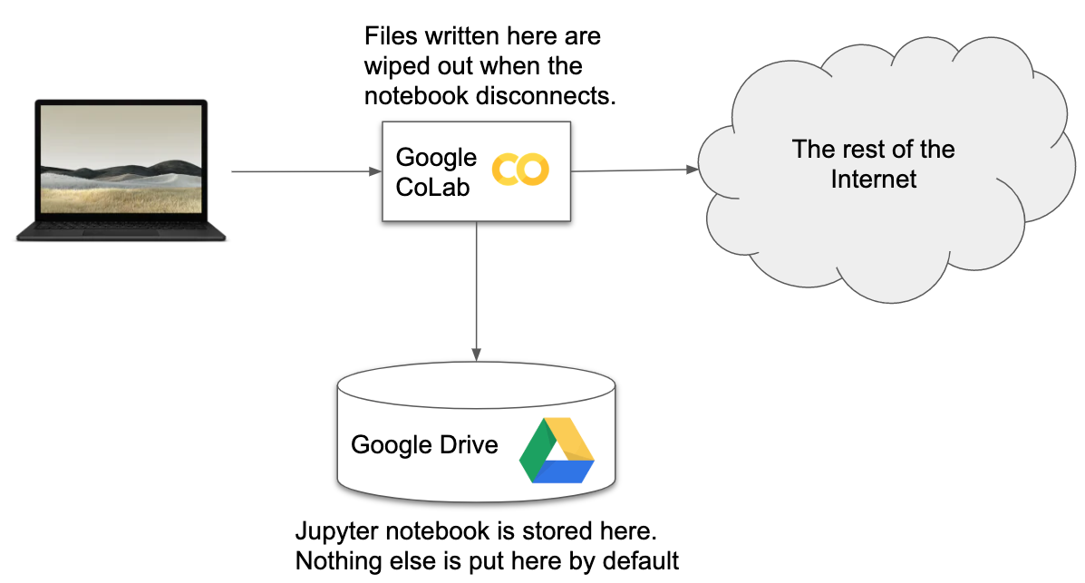
We're going to focus on 2 evironments (CoLab and MSI). There are many others. You can run a Jupyter notebook on your own laptop or you can use other online environment like Microsoft Azure Notebooks https://notebooks.azure.com
Moving Files
from google.colab import drive
drive.mount('/content/gdrive')
!ls /content/gdrive/
!ls "/content/gdrive/Shared drives"
Now, lets create a file and put it in our GDrive to make sure it's working.
!echo woo hoo > /tmp/test.txt
!mkdir -p "/content/gdrive/My Drive/csci-5980"
!cp /tmp/test.txt "/content/gdrive/My Drive/csci-5980"
Using this connection to GDrive, we can pull data into our colab instance. Another
!wget https://opendata.arcgis.com/datasets/38cfcfe07c2543ad869c8ee8c8378b5e_0.csv
now lets open it
import pandas as pd
pd.read_csv('38cfcfe07c2543ad869c8ee8c8378b5e_0.csv')
Lets try another method for getting data to our colab instance
from google.colab import files
uploaded = files.upload()
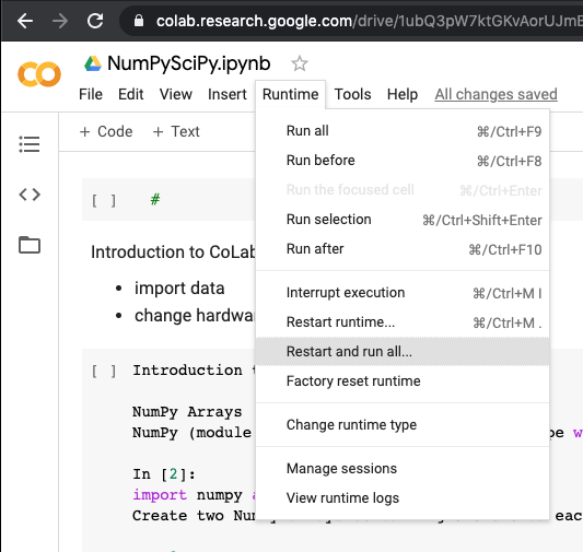
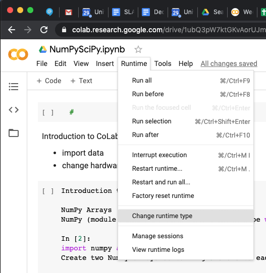
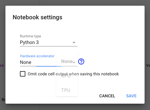
If our instance is running on a GPU, we can take a peek at what hardware we have.
!nvidia-smi
You can download your notebook from File -> Download .ipynb

This might be the easiest way to copy your notebook and move it to another platform. In addition to downloading the notebook, you can download data that you generate. E.g.;
!ls
from google.colab import files
files.download('Original-Joan-Miro-Signed-Limited-Edition.jpg')
!ls -l
Introduction to NumPy NumPy Arrays NumPy (module numpy) provides an array datatype with vectorized operations (similar to Matlab or IDL)
!pip install tensorflow
import numpy as np
Create two NumPy arrays containing 5 elements each. The numpy module contains a number of functions for generating common arrays:
x = np.arange(5)
x
y = np.ones(5)
y
Operations are vectorized, so we can do arithmetic with arrays (as long as the dimensions match!) as we would with scalar variables.
x - (y+0.005) * 3
You can try to put different types of objects into an array, and NumPy will pick a data type that can hold them all.
The results might not be quite what you expect!
mixed = np.array([3,3.3e-10,"string",5,5])
mixed
mixed*5
More sensibly, it will choose types to avoid losing precision.
z = np.array([5,6.66666666666,7,8,9],dtype=np.float32)
np.set_printoptions(precision=12)
print(z)
z.dtype
Supports the same type of list operations as ordinary Python lists:
sorted(x - y * 3)
...except the data type must match! A NumPy array only holds values of a single data type.
This allows them to be packed efficiently in memory like C arrays
y.dtype
Speed comparison Math with NumPy arrays is much faster and more intuitive than the equivalent native Python operations
Consider the function $y = 1.324\cdot a - 12.99\cdot b + 1$ In pure Python we would define:
def py_add(a, b):
    assert(len(a) == len(b))
    c = [0]*len(a)
    for i in range(0,len(a)):
        c[i] = 1.324 * a[i] - 12.99*b[i] + 1
    return c
Using NumPy we could instead define:
def np_add(a, b):
    return 1.324 * a - 12.99 * b + 1
Now let's create a couple of very large arrays to work with:
a = np.arange(1000000)
b = np.random.randn(1000000)
len(a)
b[0:20]
Use the magic function %timeit to test the performance of both approaches.
%timeit py_add(a,b)
%timeit np_add(a,b)
Now, we want to try out a memory profiler.
!pip install memory_profiler
import memory_profiler
Oops, we don't have one installed. We can install it on-the-fly like this:
import memory_profiler
%load_ext memory_profiler
%memit py_add(a,b)
%memit np_add(a,b)
Spiral Data Classification
First, we import some modules and generate data in 3 classes
%matplotlib inline
import matplotlib
from IPython.display import HTML, display, Image
import numpy as np
import matplotlib.pyplot as plt
plt.rcParams['figure.figsize'] = (12.0, 10.0) # set default size of plots
plt.rcParams['image.interpolation'] = 'nearest'
plt.rcParams['image.cmap'] = 'gray'

N = 100 # number of points per class
D = 2 # dimensionality
K = 3 # number of classes
X = np.zeros((N*K,D)) # data matrix (each row = single example)
y = np.zeros(N*K, dtype='uint8') # class labels
for j in range(K):
  ix = range(N*j,N*(j+1))
  r = np.linspace(0.0,1,N) # radius
  t = np.linspace(j*4,(j+1)*4,N) + np.random.randn(N)*0.2 # theta
  X[ix] = np.c_[r*np.sin(t), r*np.cos(t)]
  y[ix] = j
Let's visualize the data
plt.scatter(X[:, 0], X[:, 1], c=y, s=40, cmap=plt.cm.Spectral)
plt.show()
W = 0.01 * np.random.randn(D,K)
b = np.zeros((1,K))
step_size = 1e-0
reg = 1e-3
Optimize the classifier using a basic gradient descent
num_examples = X.shape[0]
for i in range(200):

  # evaluate class scores, [N x K]
  scores = np.dot(X, W) + b

  # compute the class probabilities
  exp_scores = np.exp(scores)
  probs = exp_scores / np.sum(exp_scores, axis=1, keepdims=True) # [N x K]

  # compute the loss: average cross-entropy loss and regularization
  correct_logprobs = -np.log(probs[range(num_examples),y])
  data_loss = np.sum(correct_logprobs)/num_examples
  reg_loss = 0.5*reg*np.sum(W*W)
  loss = data_loss + reg_loss
  if i % 10 == 0:
    print("iteration %d: loss %f" % (i, loss))
  # Compute the gradient
  dscores = probs
  dscores[range(num_examples),y] -= 1
  dscores /= num_examples

  # backpropogate the gradient to the parameters (W,b)
  dW = np.dot(X.T, dscores)
  db = np.sum(dscores, axis=0, keepdims=True)

  dW += reg*W # regularization gradient

  # perform a parameter update
  W += -step_size * dW
  b += -step_size * db
Evaluate the accuracy
scores = np.dot(X, W) + b
predicted_class = np.argmax(scores, axis=1)
print('training accuracy: %.2f' % (np.mean(predicted_class == y)))
print(W.size)
print(b.size)
Plot the resulting classifier
h = 0.02
x_min, x_max = X[:, 0].min() - 1, X[:, 0].max() + 1
y_min, y_max = X[:, 1].min() - 1, X[:, 1].max() + 1
xx, yy = np.meshgrid(np.arange(x_min, x_max, h),
                     np.arange(y_min, y_max, h))
Z = np.dot(np.c_[xx.ravel(), yy.ravel()], W) + b
Z = np.argmax(Z, axis=1)
Z = Z.reshape(xx.shape)
fig = plt.figure()
plt.contourf(xx, yy, Z, cmap=plt.cm.Spectral, alpha=0.8)
plt.scatter(X[:, 0], X[:, 1], c=y, s=40, cmap=plt.cm.Spectral)
plt.xlim(xx.min(), xx.max())
plt.ylim(yy.min(), yy.max())
h = 100 # size of hidden layer
W = 0.01 * np.random.randn(D,h)
b = np.zeros((1,h))
W2 = 0.01 * np.random.randn(h,K)
b2 = np.zeros((1,K))

step_size = 1e-0
reg = 1e-3 # regularization strength

# gradient descent loop
num_examples = X.shape[0]
for i in range(10000):

  # evaluate class scores, [N x K]
  hidden_layer = np.maximum(0, np.dot(X, W) + b) # note, ReLU activation
  scores = np.dot(hidden_layer, W2) + b2

  # compute the class probabilities
  exp_scores = np.exp(scores)
  probs = exp_scores / np.sum(exp_scores, axis=1, keepdims=True) # [N x K]

  # compute the loss: average cross-entropy loss and regularization
  correct_logprobs = -np.log(probs[range(num_examples),y])
  data_loss = np.sum(correct_logprobs)/num_examples
  reg_loss = 0.5*reg*np.sum(W*W) + 0.5*reg*np.sum(W2*W2)
  loss = data_loss + reg_loss
  if i % 1000 == 0:
    print("iteration %d: loss %f" % (i, loss))

  # compute the gradient on scores
  dscores = probs
  dscores[range(num_examples),y] -= 1
  dscores /= num_examples

  # backpropate the gradient to the parameters
  # first backprop into parameters W2 and b2
  dW2 = np.dot(hidden_layer.T, dscores)
  db2 = np.sum(dscores, axis=0, keepdims=True)
  # next backprop into hidden layer
  dhidden = np.dot(dscores, W2.T)
  # backprop the ReLU non-linearity
  dhidden[hidden_layer <= 0] = 0
  # finally into W,b
  dW = np.dot(X.T, dhidden)
  db = np.sum(dhidden, axis=0, keepdims=True)

  # add regularization gradient contribution
  dW2 += reg * W2
  dW += reg * W

  # perform a parameter update
  W += -step_size * dW
  b += -step_size * db
  W2 += -step_size * dW2
  b2 += -step_size * db2
Evaluate training set accuracy
hidden_layer = np.maximum(0, np.dot(X, W) + b)
scores = np.dot(hidden_layer, W2) + b2
predicted_class = np.argmax(scores, axis=1)
print('training accuracy: %.2f' % (np.mean(predicted_class == y)))
print(b.size)
print(W.size)
print(b2.size)
print(W2.size)
print(dscores.size)
Plot the resulting classifier
h = 0.02
x_min, x_max = X[:, 0].min() - 1, X[:, 0].max() + 1
y_min, y_max = X[:, 1].min() - 1, X[:, 1].max() + 1
xx, yy = np.meshgrid(np.arange(x_min, x_max, h),
                     np.arange(y_min, y_max, h))
Z = np.dot(np.maximum(0, np.dot(np.c_[xx.ravel(), yy.ravel()], W) + b), W2) + b2
Z = np.argmax(Z, axis=1)
Z = Z.reshape(xx.shape)
fig = plt.figure()
plt.contourf(xx, yy, Z, cmap=plt.cm.Spectral, alpha=0.8)
plt.scatter(X[:, 0], X[:, 1], c=y, s=40, cmap=plt.cm.Spectral)
plt.xlim(xx.min(), xx.max())
plt.ylim(yy.min(), yy.max())
Hooray, with 603 parameters, we were able to fit the data.
Introduction to SciPy
SciPy has loads of useful
- scipy.io.matlab – support for Matlab (.mat)
- scipy.io.loadmat() and scipy.io.savemat()
- Clustering algorithms (scipy.cluster)
- Integration and ODEs (scipy.integrate)
- Interpolation (scipy.interpolate)
- Input and output (scipy.io)
- Linear algebra (scipy.linalg)
- Muli-dimensional image processing (scipy.ndimage)
- Optimizaton and root finding (scipy.optimize)
- Signal processing (scipy.signal)
- Sparse matrices (scipy.sparse)
- Spatial algorithms and data structures (scipy.spatial)
- Special functions (scipy.special)
- Statstical functions (scipy.stats)
https://docs.scipy.org/doc/scipy/reference/tutorial/interpolate.html
1-D interpolation (interp1d) The interp1d class in scipy.interpolate is a convenient method to create a function based on fixed data points, which can be evaluated anywhere within the domain defined by the given data using linear interpolation. An instance of this class is created by passing the 1-D vectors comprising the data. The instance of this class defines a call method and can therefore by treated like a function which interpolates between known data values to obtain unknown values (it also has a docstring for help). Behavior at the boundary can be specified at instantiation time. The following example demonstrates its use, for linear and cubic spline interpolation:
from scipy.interpolate import interp1d

x = np.linspace(0, 10, num=11, endpoint=True)
y = np.cos(-x**2/9.0)
f = interp1d(x, y)
f2 = interp1d(x, y, kind='cubic')

xnew = np.linspace(0, 10, num=41, endpoint=True)
import matplotlib.pyplot as plt
plt.plot(x, y, 'o', xnew, f(xnew), '-', xnew, f2(xnew), '--')
plt.legend(['data', 'linear', 'cubic'], loc='best')
plt.show()
Multivariate data interpolation (griddata) Suppose you have multidimensional data, for instance, for an underlying function f(x, y) you only know the values at points (x[i], y[i]) that do not form a regular grid.
Suppose we want to interpolate the 2-D function
def func(x, y):
  return x*(1-x)*np.cos(4*np.pi*x) * np.sin(4*np.pi*y**2)**2
on a grid in [0, 1]x[0, 1]
grid_x, grid_y = np.mgrid[0:1:100j, 0:1:200j]
but we only know its values at 1000 data points:
points = np.random.rand(1000, 2)
values = func(points[:,0], points[:,1])
This can be done with the griddata function. Below, we try out all of the interpolation methods.
from scipy.interpolate import griddata
grid_z0 = griddata(points, values, (grid_x, grid_y), method='nearest')
grid_z1 = griddata(points, values, (grid_x, grid_y), method='linear')
grid_z2 = griddata(points, values, (grid_x, grid_y), method='cubic')
One can see that the exact result is reproduced by all of the methods to some degree.
import matplotlib.pyplot as plt
plt.subplot(221)
plt.imshow(func(grid_x, grid_y).T, extent=(0,1,0,1), origin='lower')
plt.plot(points[:,0], points[:,1], 'k.', ms=1)
plt.title('Original')
plt.subplot(222)
plt.imshow(grid_z0.T, extent=(0,1,0,1), origin='lower')
plt.title('Nearest')
plt.subplot(223)
plt.imshow(grid_z1.T, extent=(0,1,0,1), origin='lower')
plt.title('Linear')
plt.subplot(224)
plt.imshow(grid_z2.T, extent=(0,1,0,1), origin='lower')
plt.title('Cubic')
plt.gcf().set_size_inches(10, 10)
plt.show()
Notebooks at MSI
Jupyter is more than an interface for teaching. Jupyter is heavily used by researchers. It's a great interface for research. MSI has a large cluster for running large-scale simulations and data anlysis. MSI also runs JupyterHub to allow researchers to access thier data in a Jupyter environment. JupyterHub can be accessed here:
To use the notebooks at MSI, you will first need to select the group you want to work in. Most of you only have access to a single group. If you happen to be doing some research, you might have access to another group. After you select the group created for the class (csci5980) and press continue, you can click a button that reads "Start My Server". This will bring you to a dropdown menu to select the resources you need.
You can select the one labeled "Mesabi - 2 Cores, 4 GB, 8 hours". This will submit a job to the cluster and reserve the described resources for your Jupyter session.
JupyterHub at MSI is being upgraded over the next few weeks, so there will be some changes and outages to the interface. Expect email with updates!